 |
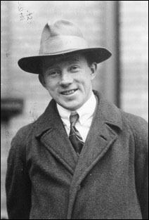
| Heisenberg, 1927 |
Click here and read for a layman's overview.

Here is the mathematics, from Wikipedia:
In quantum mechanics, the Heisenberg uncertainty principle states by precise inequalities that certain pairs of physical properties, such as position and momentum, cannot be simultaneously known to arbitrarily high precision. That is, the more precisely one property is measured, the less precisely the other can be measured.
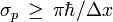
Published by Werner Heisenberg in 1927, the principle means that it is impossible to determine simultaneously both the position and the momentum of an electron or any other particle with any great degree of accuracy or certainty. This is not a statement about researchers' ability to measure the quantities. Rather, it is a statement about the system itself. That is, a system cannot be defined to have simultaneously singular values of these pairs of quantities. The principle states that a minimum exists for the product of the uncertainties in these properties that is equal to or greater than one half of the reduced Planck constant (ħ = h/2π).
In quantum physics, a particle is described by a wave packet, which gives rise to this phenomenon. Consider the measurement of the position of a particle. It could be anywhere. The particle's wave packet has non-zero amplitude, meaning the position is uncertain – it could be almost anywhere along the wave packet. To obtain an accurate reading of position, this wave packet must be 'compressed' as much as possible, meaning it must be made up of increasing numbers of sine waves added together. The momentum of the particle is proportional to the wavenumber of one of these waves, but it could be any of them. So a more precise position measurement – by adding together more waves – means the momentum measurement becomes less precise (and vice versa).
The only kind of wave with a definite position is concentrated at one point, and such a wave has an indefinite wavelength (and therefore an indefinite momentum). Conversely, the only kind of wave with a definite wavelength is an infinite regular periodic oscillation over all space, which has no definite position. So in quantum mechanics, there can be no states that describe a particle with both a definite position and a definite momentum. The more precise the position, the less precise the momentum.
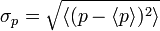
A mathematical statement of the principle is that every quantum state has the property that the root mean square (RMS) deviation of the position from its mean (the standard deviation of the x-distribution):


-
-
 .
.
-
Contents |
Historical introduction
Main article: Introduction to quantum mechanics
Werner Heisenberg formulated the uncertainty principle at Niels Bohr's institute in Copenhagen, while working on the mathematical foundations of quantum mechanics.In 1925, following pioneering work with Hendrik Kramers, Heisenberg developed matrix mechanics, which replaced the ad-hoc old quantum theory with modern quantum mechanics. The central assumption was that the classical motion was not precise at the quantum level, and electrons in an atom did not travel on sharply defined orbits. Rather, the motion was smeared out in a strange way: the Fourier transform of time only involving those frequencies that could be seen in quantum jumps.
Heisenberg's paper did not admit any unobservable quantities like the exact position of the electron in an orbit at any time; he only allowed the theorist to talk about the Fourier components of the motion. Since the Fourier components were not defined at the classical frequencies, they could not be used to construct an exact trajectory, so that the formalism could not answer certain overly precise questions about where the electron was or how fast it was going.
The most striking property of Heisenberg's infinite matrices for the position and momentum is that they do not commute. Heisenberg's canonical commutation relation indicates by how much:
-
-
![[X,P] = X P - P X = i \hbar](http://upload.wikimedia.org/math/0/3/4/0342ffe593429f253ff09a217ad29be5.png) (see derivations below)
(see derivations below)
-
In March 1926, working in Bohr's institute, Heisenberg realized that the non-commutativity implies the uncertainty principle. This was a clear physical interpretation for the non-commutativity, and it laid the foundation for what became known as the Copenhagen interpretation of quantum mechanics. Heisenberg showed that the commutation relation implies an uncertainty, or in Bohr's language a complementarity.[1] Any two variables that do not commute cannot be measured simultaneously—the more precisely one is known, the less precisely the other can be known.
One way to understand the complementarity between position and momentum is by wave-particle duality. If a particle described by a plane wave passes through a narrow slit in a wall like a water-wave passing through a narrow channel, the particle diffracts and its wave comes out in a range of angles. The narrower the slit, the wider the diffracted wave and the greater the uncertainty in momentum afterwards. The laws of diffraction require that the spread in angle Δθ is about λ / d, where d is the slit width and λ is the wavelength. From the de Broglie relation, the size of the slit and the range in momentum of the diffracted wave are related by Heisenberg's rule:


A rigorous proof of a new inequality for simultaneous measurements in the spirit of Heisenberg and Bohr has been given recently. The measurement process is as follows: Whenever a particle is localized in a finite interval Δx > 0, then the standard deviation of its momentum satisfies

Terminology
Throughout the main body of his original 1927 paper, written in German, Heisenberg used the word "Unbestimmtheit" ("indeterminacy") to describe the basic theoretical principle. Only in the endnote did he switch to the word "Unsicherheit" ("uncertainty"). However, when the English-language version of Heisenberg's textbook, The Physical Principles of the Quantum Theory, was published in 1930, the translation "uncertainty" was used, and it became the more commonly used term in the English language thereafter.[6]
Heisenberg's microscope

Main article: Heisenberg's microscope
One way in which Heisenberg originally argued for the uncertainty principle is by using an imaginary microscope as a measuring device.[3] He imagines an experimenter trying to measure the position and momentum of an electron by shooting a photon at it.If the photon has a short wavelength, and therefore a large momentum, the position can be measured accurately. But the photon scatters in a random direction, transferring a large and uncertain amount of momentum to the electron. If the photon has a long wavelength and low momentum, the collision doesn't disturb the electron's momentum very much, but the scattering will reveal its position only vaguely.
If a large aperture is used for the microscope, the electron's location can be well resolved (see Rayleigh criterion); but by the principle of conservation of momentum, the transverse momentum of the incoming photon and hence the new momentum of the electron resolves poorly. If a small aperture is used, the accuracy of the two resolutions is the other way around.
The trade-offs imply that no matter what photon wavelength and aperture size are used, the product of the uncertainty in measured position and measured momentum is greater than or equal to a lower bound, which is up to a small numerical factor equal to Planck's constant.[7] Heisenberg did not care to formulate the uncertainty principle as an exact bound, and preferred to use it as a heuristic quantitative statement, correct up to small numerical factors.
Critical reactions
Main article: Bohr–Einstein debates
The Copenhagen interpretation of quantum mechanics and Heisenberg's Uncertainty Principle were in fact seen as twin targets by detractors who believed in an underlying determinism and realism. Within the Copenhagen interpretation of quantum mechanics, there is no fundamental reality the quantum state describes, just a prescription for calculating experimental results. There is no way to say what the state of a system fundamentally is, only what the result of observations might be.Albert Einstein believed that randomness is a reflection of our ignorance of some fundamental property of reality, while Niels Bohr believed that the probability distributions are fundamental and irreducible, and depend on which measurements we choose to perform. Einstein and Bohr debated the uncertainty principle for many years.
Einstein's slit
The first of Einstein's thought experiments challenging the uncertainty principle went as follows:
- Consider a particle passing through a slit of width d. The slit introduces an uncertainty in momentum of approximately h/d because the particle passes through the wall. But let us determine the momentum of the particle by measuring the recoil of the wall. In doing so, we find the momentum of the particle to arbitrary accuracy by conservation of momentum.
A similar analysis with particles diffracting through multiple slits is given by Richard Feynman.[8]
Einstein's box
Another of Einstein's thought experiments (Einstein's box) was designed to challenge the time/energy uncertainty principle. It is very similar to the slit experiment in space, except here the narrow window the particle passes through is in time:
- Consider a box filled with light. The box has a shutter that a clock opens and quickly closes at a precise time, and some of the light escapes. We can set the clock so that the time that the energy escapes is known. To measure the amount of energy that leaves, Einstein proposed weighing the box just after the emission. The missing energy lessens the weight of the box. If the box is mounted on a scale, it is naively possible to adjust the parameters so that the uncertainty principle is violated.
EPR paradox for entangled particles
Bohr was compelled to modify his understanding of the uncertainty principle after another thought experiment by Einstein. In 1935, Einstein, Podolsky and Rosen (see EPR paradox) published an analysis of widely separated entangled particles. Measuring one particle, Einstein realized, would alter the probability distribution of the other, yet here the other particle could not possibly be disturbed. This example led Bohr to revise his understanding of the principle, concluding that the uncertainty was not caused by a direct interaction.[9]
But Einstein came to much more far-reaching conclusions from the same thought experiment. He believed as "natural basic assumption" that a complete description of reality would have to predict the results of experiments from "locally changing deterministic quantities", and therefore would have to include more information than the maximum possible allowed by the uncertainty principle.
In 1964 John Bell showed that this assumption can be falsified, since it would imply a certain inequality between the probabilities of different experiments. Experimental results confirm the predictions of quantum mechanics, ruling out Einstein's basic assumption that led him to the suggestion of his hidden variables. (Ironically this is one of the best examples for Karl Popper's philosophy of invalidation of a theory by falsification-experiments; i.e. here Einstein's "basic assumption" became falsified by experiments based on Bell's inequalities; for the objections of Karl Popper against the Heisenberg inequality itself, see below.)
While it is possible to assume that quantum mechanical predictions are due to nonlocal hidden variables, and in fact David Bohm invented such a formulation, this is not a satisfactory resolution for the vast majority of physicists. The question of whether a random outcome is predetermined by a nonlocal theory can be philosophical, and potentially intractable. If the hidden variables are not constrained, they could just be a list of random digits that are used to produce the measurement outcomes. To make it sensible, the assumption of nonlocal hidden variables is sometimes augmented by a second assumption — that the size of the observable universe puts a limit on the computations that these variables can do. A nonlocal theory of this sort predicts that a quantum computer encounters fundamental obstacles when it tries to factor numbers of approximately 10,000 digits or more; an achievable task in quantum mechanics.[10]
Popper's criticism
Karl Popper criticized Heisenberg's form of the uncertainty principle, that a measurement of position disturbs the momentum, based on the following observation: if a particle with definite momentum passes through a narrow slit, the diffracted wave has some amplitude to go in the original direction of motion. If the momentum of the particle is measured after it goes through the slit, there is always some probability, however small, that the momentum will be the same as it was before.
Popper thinks of these rare events as falsifications of the uncertainty principle in Heisenberg's original formulation. To preserve the principle, he concludes that Heisenberg's relation does not apply to individual particles or measurements, but only to many identically prepared particles, called ensembles. Popper's criticism applies to nearly all probabilistic theories, since a probabilistic statement requires many measurements to either verify or falsify.
Popper's criticism does not trouble physicists who subscribe to the Copenhagen interpretation of Quantum Mechanics. Popper's presumption is that the measurement is revealing some preexisting information about the particle, the momentum, which the particle already possesses. According to the Copenhagen interpretation, the quantum mechanical description of the wavefunction is not a reflection of ignorance about the values of some more fundamental quantities; it is the complete description of the state of the particle. In this philosophical view, Popper's example is not a falsification, since after the particle diffracts through the slit and before the momentum is measured, the wavefunction is changed so that the momentum is still as uncertain as the principle demands.
Mathematical derivations
When linear operators A and B act on a function ψ(x), they don't always commute. A clear example is when operator B multiplies x, while operator A takes the derivative with respect to x. Then, for every wave function ψ(x) we can write


 , so that:
![[p,x] = p x - x p = -i\hbar \left( {d\over dx} x - x {d\over dx} \right) = - i \hbar.](http://upload.wikimedia.org/math/e/2/0/e209eb230eb1a01899da35b25da38e24.png)
For any two operators A and B:

 and
and  . On the other hand, the expectation value of the product AB is always greater than the magnitude of its imaginary part:
![\langle A^2 \rangle \langle B^2 \rangle\ge {1\over 4} |\langle [A,B]\rangle|^2](http://upload.wikimedia.org/math/e/a/9/ea96244c63616b1e0a3d9e7868a90223.png)
Physical Interpretation
The inequality above acquires its dispersion interpretation:
![\sigma_A\sigma_B \ge \frac{1}{2} \left|\left\langle\left[{A},{B}\right]\right\rangle\right|](http://upload.wikimedia.org/math/f/8/3/f8393ca8b47169c71f08ca74d35cce41.png)


By substituting
 for A and
  for B in the general operator norm inequality, since the imaginary part of the product, the commutator is unaffected by the shift:
![[A - \lang A\rang, B - \lang B\rang] = [ A , B ].](http://upload.wikimedia.org/math/c/1/2/c12f985e7adaf649217b038c4c613295.png) and , which in quantum mechanics are the standard deviations of A and B. The small side is the norm of the commutator, which for the position and momentum is just
and , which in quantum mechanics are the standard deviations of A and B. The small side is the norm of the commutator, which for the position and momentum is just  .
.A further generalization is due to Schrödinger: Given any two Hermitian operators A and B, and a system in the state ψ, there are probability distributions for the value of a measurement of A and B, with standard deviations σA and σB. Then
![\sigma_A \sigma_B \geq \sqrt{ \frac{1}{4}\left|\left\langle\left[{A},{B}\right]\right\rangle\right|^2
+{1\over 4} \left|\left\langle\left\{ A-\langle A\rangle,B-\langle B\rangle \right\} \right\rangle \right|^2}](http://upload.wikimedia.org/math/f/a/2/fa233527d3f84d7356824a9a9a448a8a.png)
Examples
The Robertson-Schrödinger relation gives the uncertainty relation for any two observables that do not commute:
- between position and momentum by applying the commutator relation
![[x,p_x]=i\hbar](http://upload.wikimedia.org/math/a/5/4/a54264a655e2e824a033aa70f53e51d5.png) :
:

- between the kinetic energy T and position x of a particle :
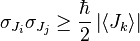
- between two orthogonal components of the total angular momentum operator of an object:
-
- where i, j, k are distinct and Ji denotes angular momentum along the xi axis. This relation implies that only a single component of a system's angular momentum can be defined with arbitrary precision, normally the component parallel to an external (magnetic or electric) field.
- between angular position and angular momentum of an object with small angular uncertainty:

- between the number of electrons in a superconductor and the phase of its Ginzburg–Landau order parameter[11][12]

Energy-time uncertainty principle
One well-known uncertainty relation is not an obvious consequence of the Robertson–Schrödinger relation: the energy-time uncertainty principle.
Since energy bears the same relation to time as momentum does to space in special relativity, it was clear to many early founders, Niels Bohr among them, that the following relation holds:[2][3]

Nevertheless, Einstein and Bohr understood the heuristic meaning of the principle. A state that only exists for a short time cannot have a definite energy. To have a definite energy, the frequency of the state must accurately be defined, and this requires the state to hang around for many cycles, the reciprocal of the required accuracy.
For example, in spectroscopy, excited states have a finite lifetime. By the time-energy uncertainty principle, they do not have a definite energy, and each time they decay the energy they release is slightly different. The average energy of the outgoing photon has a peak at the theoretical energy of the state, but the distribution has a finite width called the natural linewidth. Fast-decaying states have a broad linewidth, while slow decaying states have a narrow linewidth.
The broad linewidth of fast decaying states makes it difficult to accurately measure the energy of the state, and researchers have even used microwave cavities to slow down the decay-rate, to get sharper peaks.[13] The same linewidth effect also makes it difficult to measure the rest mass of fast decaying particles in particle physics. The faster the particle decays, the less certain is its mass.
One false formulation of the energy-time uncertainty principle says that measuring the energy of a quantum system to an accuracy ΔE requires a time interval Δt > h / ΔE. This formulation is similar to the one alluded to in Landau's joke, and was explicitly invalidated by Y. Aharonov and D. Bohm in 1961. The time Δt in the uncertainty relation is the time during which the system exists unperturbed, not the time during which the experimental equipment is turned on.
Another common misconception is that the energy-time uncertainty principle says that the conservation of energy can be temporarily violated – energy can be "borrowed" from the Universe as long as it is "returned" within a short amount of time.[14] Although this agrees with the spirit of relativistic quantum mechanics, it is based on the false axiom that the energy of the Universe is an exactly known parameter at all times. More accurately, when events transpire at shorter time intervals, there is a greater uncertainty in the energy of these events. Therefore it is not that the conservation of energy is violated when quantum field theory uses temporary electron-positron pairs in its calculations, but that the energy of quantum systems is not known with enough precision to limit their behavior to a single, simple history. Thus the influence of all histories must be incorporated into quantum calculations, including those with much greater or much less energy than the mean of the measured/calculated energy distribution.
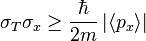
In 1936 Dirac offered a precise definition and derivation of the time-energy uncertainty relation in a relativistic quantum theory of "events".[citation needed] But a better-known, more widely used formulation of the time-energy uncertainty principle was given in 1945 by L. I. Mandelshtam and I. E. Tamm, as follows.[15] For a quantum system in a non-stationary state ψ and an observable B represented by a self-adjoint operator
 , the following formula holds:
 changes appreciably.
Entropic uncertainty principle
Main article: Hirschman uncertainty
While formulating the many-worlds interpretation of quantum mechanics in 1957, Hugh Everett III discovered a much stronger formulation of the uncertainty principle.[16] In the inequality of standard deviations, some states, like the wavefunction

Taking the logarithm of Heisenberg's formulation of uncertainty in natural units.

Everett (and Hirschman[17]) conjectured that for all quantum states:

Uncertainty theorems in harmonic analysis
In the context of harmonic analysis, the uncertainty principle implies that one cannot at the same time localize the value of a function and its Fourier transform; to wit, the following inequality holds

Benedicks's theorem
Amrein-Berthier (Amrein & Berthier 1977) and Benedicks's theorem (Benedicks 1985) intuitively says that the set of points where ƒ is non-zero and the set of points where
 is nonzero cannot both be small. Specifically, it is impossible for a function ƒ in L2(R) and its Fourier transform to both be supported on sets of finite Lebesgue measure. In signal processing, this includes the following well-known result: a function cannot be both time limited and band limited. A more quantitative version is due to Nazarov (Nazarov 1994) and (Jaming 2007):
One expects that the factor CeC | S | | Σ | may be replaced by
 which is only known if either S or Σ is convex.
Hardy's uncertainty principle
The mathematician G. H. Hardy (Hardy 1933) formulated the following uncertainty principle: it is not possible for ƒ and
to both be "very rapidly decreasing." Specifically, if ƒ is in L2(R), is such that  and
and  (C > 0,N an integer) then, if ab > 1,f = 0 while if ab = 1 then there is a polynomial P of degree
  such that
 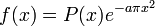 . This was later improved as follows: if
  is such that
 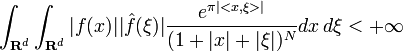 then, f(x) = P(x)e − π < Ax,x > where P is a polynomial of degree
  and A is a real
  positive definite matrix.
This result was stated in Beurling's complete works without proof and proved in Hörmander (Hörmander 1991) (the case d = 1,N = 0) and Bonami–Demange–Jaming (Bonami, Demange & Jaming 2003) for the general case.
Note that Hörmander–Beurling's version implies the case ab > 1 in Hardy's Theorem while the version by Bonami–Demange–Jaming covers the full strength of Hardy's Theorem. A full description of the case ab < 1 as well as the following extension to Schwarz class distributions appears in Demange (Demange 2010): if
 is such that
  and
and  then f(x) = P(x)e − π < Ax,x > where P is a polynomial and A is a real positive definite matrix.
Uncertainty principle of game theory
The uncertainty principle of game theory was formulated by Szekely and Rizzo in 2007.[19] This principle is a lower bound for the entropy of optimal strategies of players in terms of the commutator of two nonlinear operators: minimum and maximum. If the payoff matrix (aij) of an arbitrary zero-sum game is normalized (i.e. the smallest number in this matrix is 0, the biggest number is 1) and the commutator
minj maxi (aij) − maxi minj (aij) = h then the entropy of the optimal strategy of any of the players cannot be smaller than the entropy of the two-point distribution [1/(1+h), h/(1+h)] and this is the best lower bound. (This is zero if and only if h = 0 i.e. if min and max are commutable in which case the game has pure nonrandom optimal strategies). As an application, one could optimize between these two-point strategies via considering the distribution [1/(1+h), h/(1+h)] on all pairs of pure strategies. In many practical cases we do not lose much by neglecting more complex strategies.
No comments:
Post a Comment